
Note
Go to the end to download the full example code.
Equations of state functions#
Machida06 EoS#
11 import matplotlib.pyplot as plt
12 import numpy as np
13
14 import shamrock
Use shamrock documentation style for matplotlib
18 shamrock.matplotlib.set_shamrock_mpl_style()
Machida06 EoS
22 cs = 190.0
23 rho_c1 = 1.92e-13 * 1000 # g/cm^3 -> kg/m^3
24 rho_c2 = 3.84e-8 * 1000 # g/cm^3 -> kg/m^3
25 rho_c3 = 1.92e-3 * 1000 # g/cm^3 -> kg/m^3
26
27
28 si = shamrock.UnitSystem()
29 sicte = shamrock.Constants(si)
30 kb = sicte.kb()
31 print(kb)
32 mu = 2.375
33 mh = 1.00784 * sicte.dalton()
34 print(mu * mh * kb)
35
36 rho_plot = np.logspace(-15, 5, 1000)
37 P_plot = []
38 cs_plot = []
39 T_plot = []
40 for rho in rho_plot:
41 P, _cs, T = shamrock.phys.eos.eos_Machida06(
42 cs=cs, rho=rho, rho_c1=rho_c1, rho_c2=rho_c2, rho_c3=rho_c3, mu=mu, mh=mh, kb=kb
43 )
44 P_plot.append(P)
45 cs_plot.append(_cs)
46 T_plot.append(T)
47
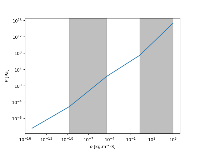
48 plt.figure()
49 plt.plot(rho_plot, P_plot, label="P")
50 plt.yscale("log")
51 plt.xscale("log")
52 plt.xlabel("$\\rho$ [kg.m^-3]")
53 plt.ylabel("$P$ [Pa]")
54 plt.axvspan(rho_c1, rho_c2, color="grey", alpha=0.5)
55 plt.axvspan(rho_c3, rho_plot[-1], color="grey", alpha=0.5)
56
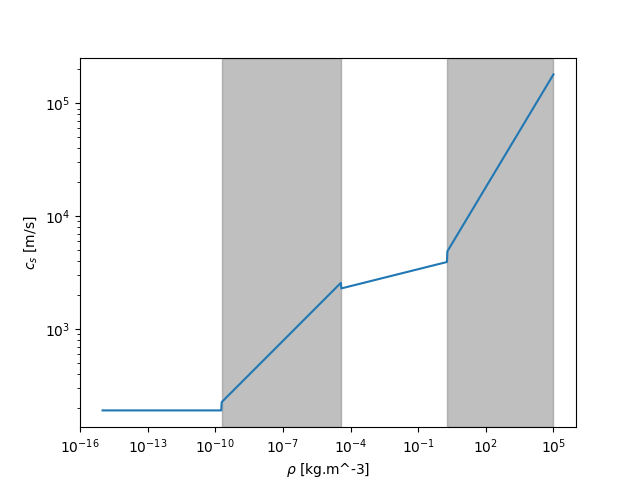
57 plt.figure()
58 plt.plot(rho_plot, cs_plot, label="cs")
59 plt.yscale("log")
60 plt.xlabel("$\\rho$ [kg.m^-3]")
61 plt.xscale("log")
62 plt.ylabel("$c_s$ [m/s]")
63 plt.axvspan(rho_c1, rho_c2, color="grey", alpha=0.5)
64 plt.axvspan(rho_c3, rho_plot[-1], color="grey", alpha=0.5)
65
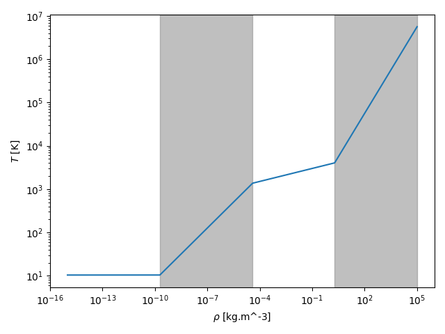
66 plt.figure()
67 plt.plot(rho_plot, T_plot, label="T")
68 plt.yscale("log")
69 plt.xscale("log")
70 plt.xlabel("$\\rho$ [kg.m^-3]")
71 plt.ylabel("$T$ [K]")
72 plt.axvspan(rho_c1, rho_c2, color="grey", alpha=0.5)
73 plt.axvspan(rho_c3, rho_plot[-1], color="grey", alpha=0.5)
74
75
76 plt.tight_layout()
1.380649e-23
5.487664926077112e-50
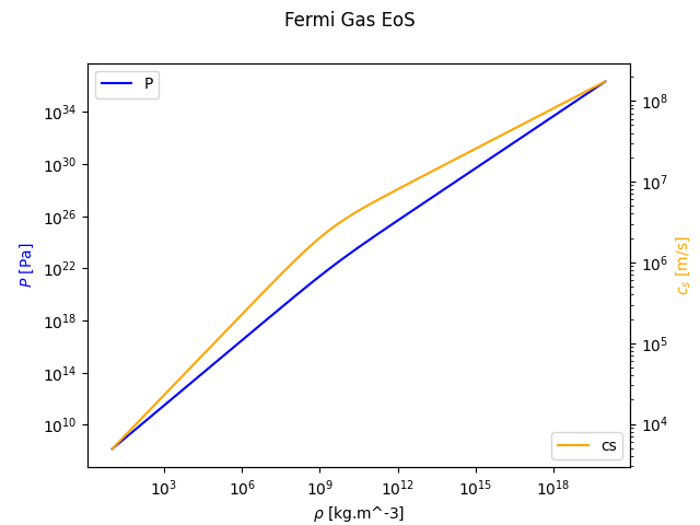
Fermi gas EoS#
 82 rho_plot = np.logspace(1, 20, 1000)
 83 P_plot = []
 84 cs_plot = []
 85
 86 for rho in rho_plot:
 87     P, _cs = shamrock.phys.eos.eos_Fermi(mu_e=2, rho=rho)
 88     P_plot.append(P)
 89     cs_plot.append(_cs)
 90
 91 plt.figure()
 92 plt.suptitle("Fermi Gas EoS")
 93 plt.plot(rho_plot, P_plot, label="P", color="blue")
 94 plt.yscale("log")
 95 plt.xscale("log")
 96 plt.xlabel("$\\rho$ [kg.m^-3]")
 97 plt.ylabel("$P$ [Pa]", color="blue")
 98 plt.legend()
 99
100
101 ax = plt.twinx()
102 ax.plot(rho_plot, cs_plot, label="cs", color="orange")
103 ax.set_yscale("log")
104 ax.set_ylabel("$c_s$ [m/s]", color="orange")
105 ax.legend(loc="lower right")
<matplotlib.legend.Legend object at 0x7fbc85bd97b0>
Total running time of the script: (0 minutes 1.200 seconds)
Estimated memory usage: 159 MB